Understanding text size and resolution in ggplot2
What’s complicated about size and resolution ?
Have you ever tried to reproduce a plot like the first one and make minor changes on the size or resolution and end up with something like the second plot ? If yes, stay with me, this is the situation we’re going to understand in this article.
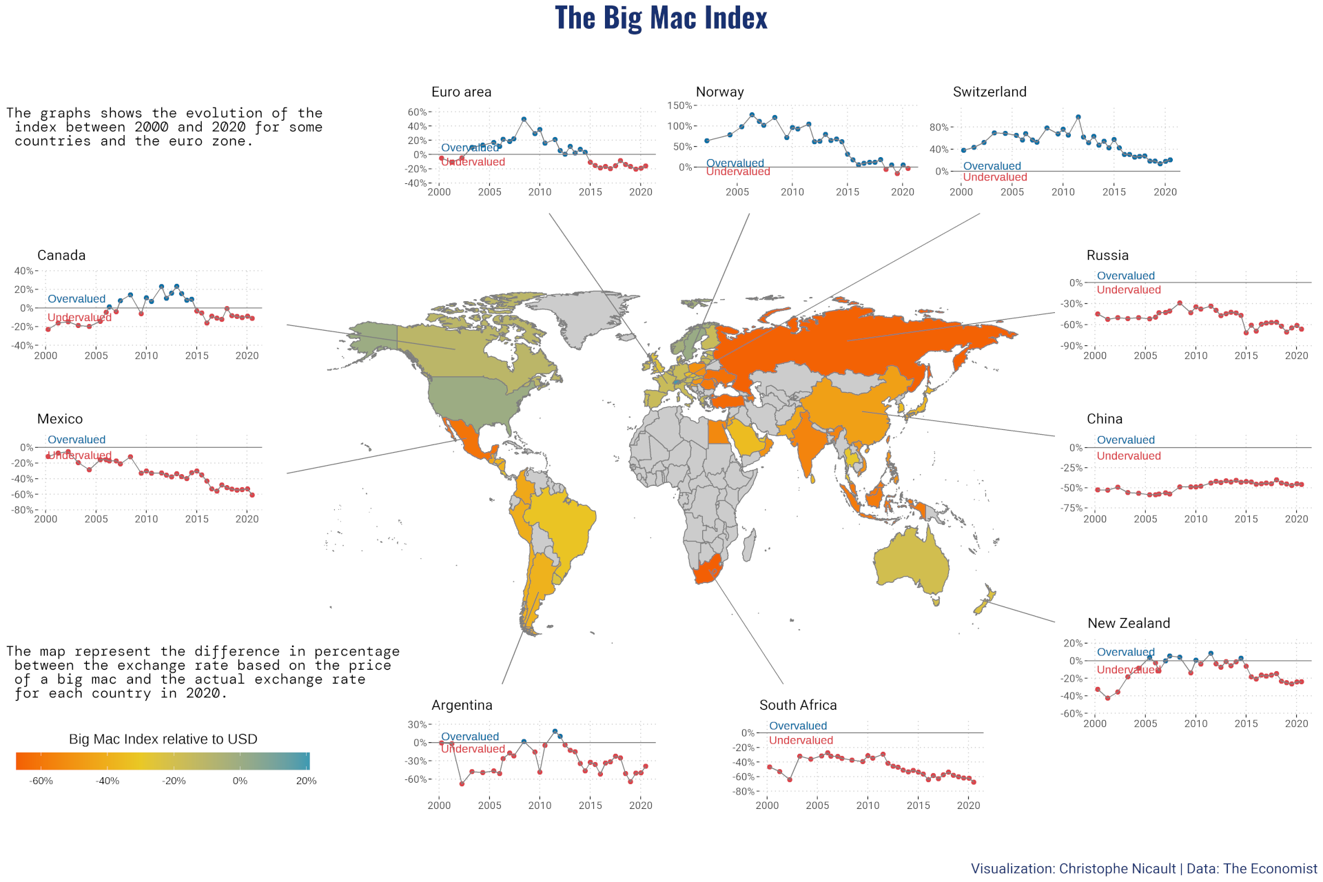
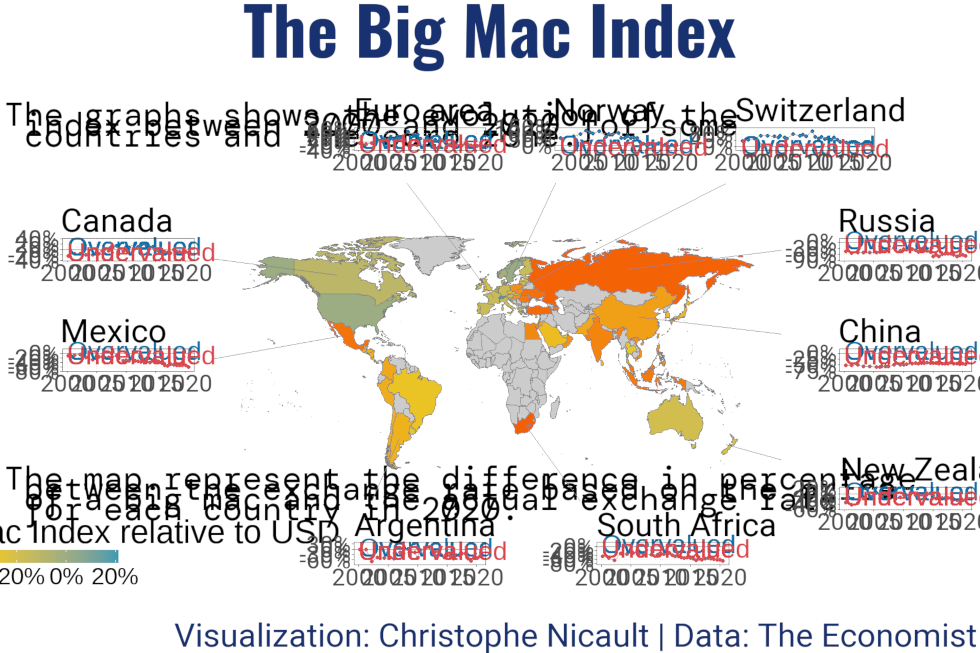
There are several things to notice :
- Obviously the font size is not the same and is a lot bigger.
- The map is a bit smaller, but still looks ok.
- The different graphs seem to be crushed, their width are the same, but not their height. In fact they seem to take the same place overall (title and axis text included) but as the font is bigger, there is less room for the graph.
- The legend doesn’t fit anymore, and is clipped.
So we’re going to see what the problem is, when it occurs, how to solve it, and more importantly how to avoid it.
Screen and image file
First let’s review some basic concepts.
Screen dimension and resolution
A screen is basically a matrix of pixels, which is the smallest element that can be displayed.
If we look at the physical dimension, my screen has a diagonal of 24 inches, with a ratio of 16/10, which is 20 x 12.5 inches.
The resolution is 1920 x 1200, my screen is a matrix of 1920 pixels width and 1200 pixels height. The number of pixels per inch is 96 (ppi).
Now we can make some calculation, everything matches :
- width : 1920 (px) / 96 (px/in) = 20 inches
- height: 1200 (px) / 96 (px/in) = 12.5 inches
- ratio: 1920/1200 = 20/12.5 = 16/10
Image files dimension and resolution
The image saved on a disk is represented also as a matrix of dots. ggplot and ggsave works in physical dimension (in, cm, or mm). To go from the dimension in inches to a number of dots, ggsave uses the number of dots per inches (dpi).
So if we create a plot in ggplot and save it with a dimension of 12 x 10 with the default dpi of 300 for ggsave, the file will be a matrix of (12 * 300) x (10 * 300) = 3600 x 3000 dots.
Now if you open that file on your computer, each dots represent a pixel, which means that the image has a resolution of 3600 x 3000 px.
The relation is : (size in inches) = (screen size in pixel) / PPI or (screen size in pixel) = DPI * (size in inches)
Let’s experiment it
We’re going to make a small experiment to understand the relation between the screen resolution and the size when saving a plot.
Let say your screen resolution is 1920*1200, the default device is almost taking all screen. The DPI for my screen is 96, so when saving to disk, we can expect the file to be saved with a dimension of 20 x 12.5 inches.
Let’s check it out :
First load the libraries and the data
library(ggplot2)
library(dplyr)
library(palmerpenguins)
theme_set(theme_bw())
Then open a new graphic device with x11() (or quartz(), or windows() depending on your system) with a dimension of 1920 x 1200.
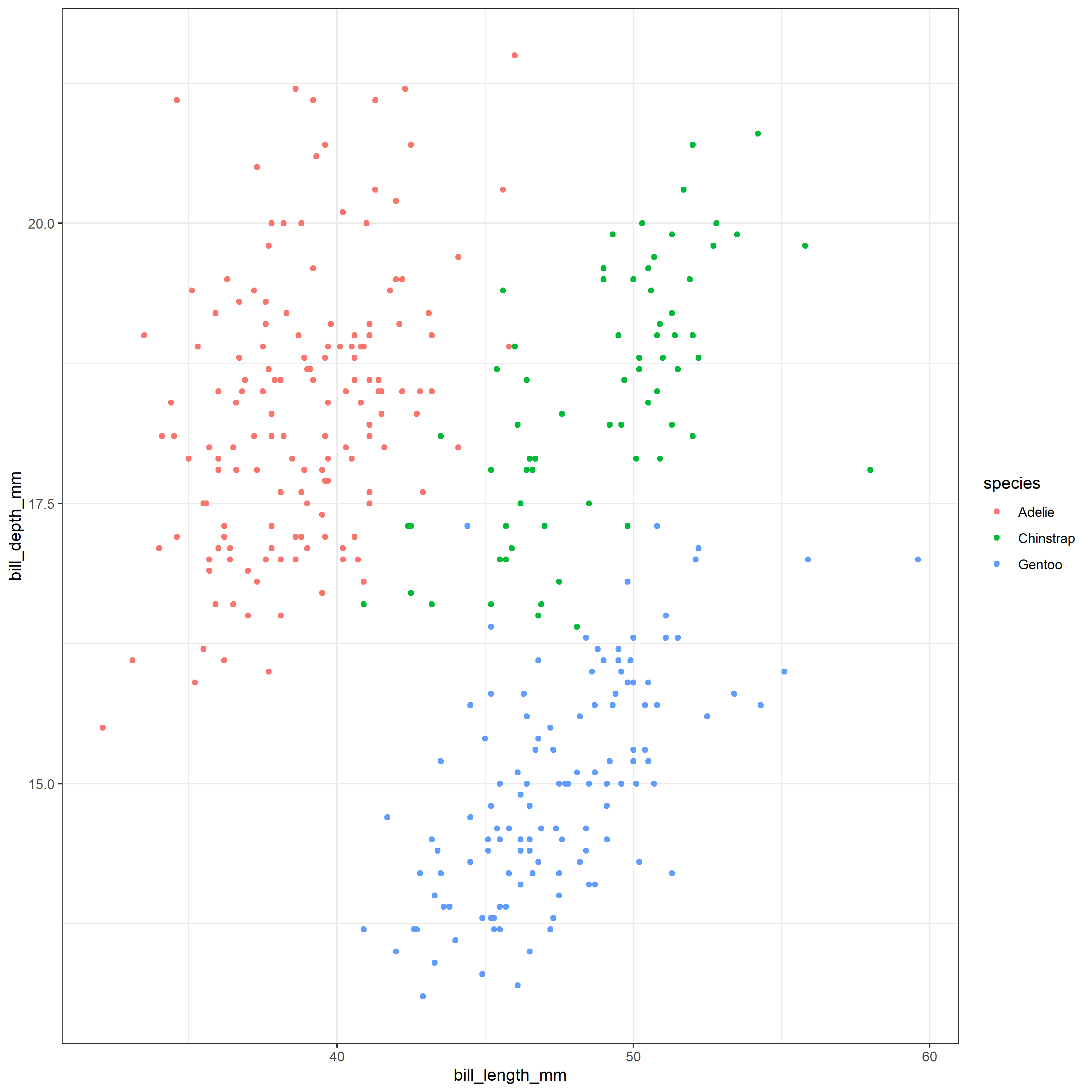
x11()Then run the following code, to create a simple plot and save it to disk.
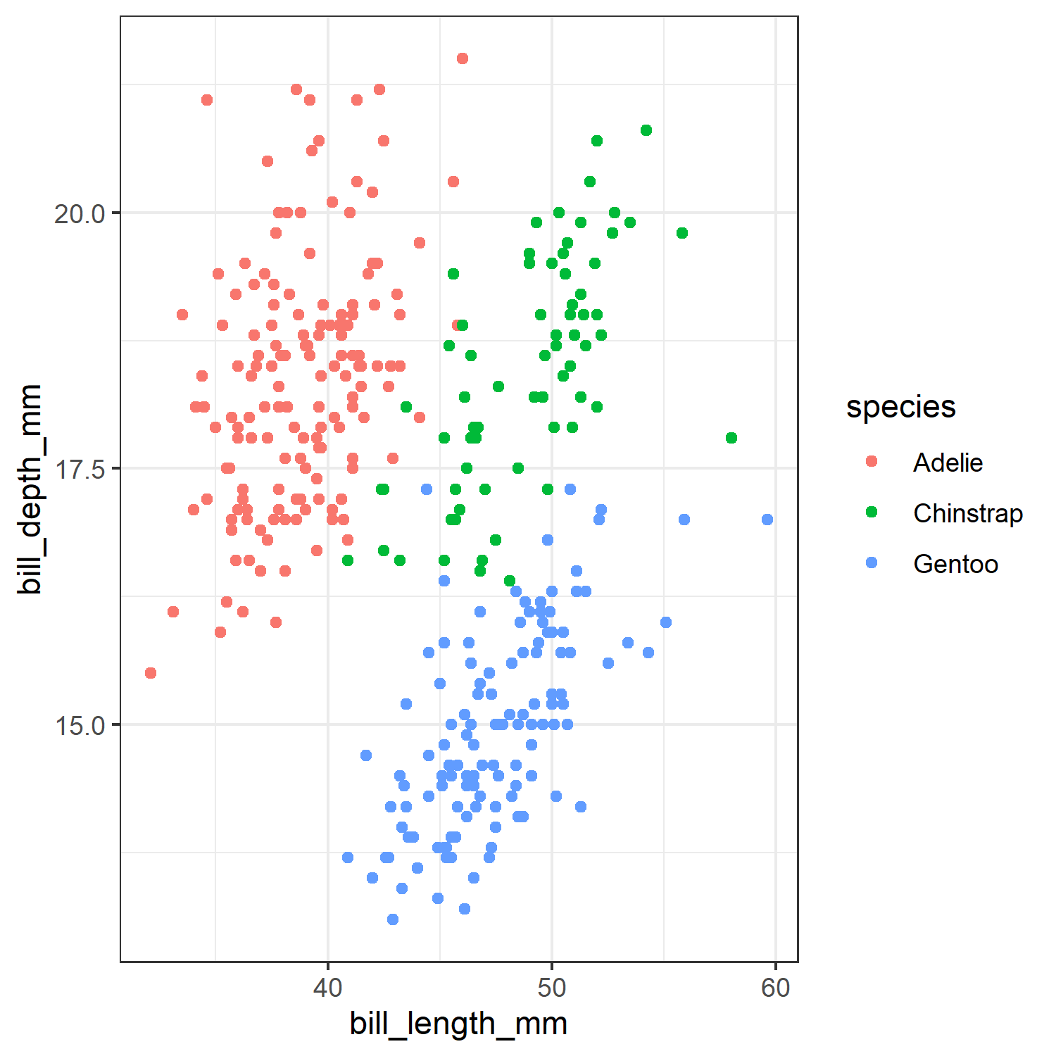
plt <- penguins %>%
  ggplot(aes(bill_length_mm, bill_depth_mm, color = species)) +
  geom_point()

ggsave("test.png")),
       plot = plt, dpi = 300)

dev.off()
You can see that the plot is saved with a size of 20 x 11.7 inches, which is the dimension of the screen (minus the window’s menu bar) divided by the default screen DPI of 96 as expected.
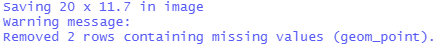
But if you check the file, you will see that the resolution is not 1920 x 1200, but 6000 x 3521 !
![]()
What happened?
The plot dimension is converted in inches before saving to disk, using the screen DPI of 96 to make the conversion (1920 / 96) x (1200 / 96) = 20 x 12.5. Then ggsave uses this dimension in inches with the DPI of 300 to save it to disk, creating an image of (20 * 300) x (12.5 * 300) = 6000 x 3510 dots.
So this is important to understand when experimenting and rendering in RStudio and then saving to disk. The relation between screen size and the physical size depend on the DPI (dot per inches) of the graphic device, which is 96 by default for the screen. Then if you save the plot with a higher or smaller DPI, the file is saved as a matrix of dots using the new DPI and the size in inches. So when opened on the computer, the size dimension in pixel is different.
Why does it matter for the original problem ?
It matters because some elements of the plot adjusts to the space available, and some are fixed and measured in their real dimension (mm, inches) such as the fonts, creating a distortion when changing the dimension of the plot or its resolution.
The font problem
Before continuing, make sure that the window we opened previously is closed.
Saving in different dimensions, the plot itself will adapt and use the full size. So for the previous plot, if we save it with 5x5 or 10x10, it works, the two plot will still look very similar
ggsave("font_test1_5x5_300.png", plot = plt, width = 5, height = 5, units = "in", dpi = 300)

ggsave("font_test1_10x10_300.png", plot = plt, width = 10, height = 10, units = "in", dpi = 300)
But we can notice that the size of the point and the size of the font looks smaller in the second one.
In fact, they are not smaller, they still have the same size in inches, and as we saved with the same resolution (dpi = 300), they have the same number of dots ( size in inches * 300). But the font appear smaller on the screen if you display the plot to fit in the screen, as the second plot is bigger (3000x3000 vs 1500 x 1500) :
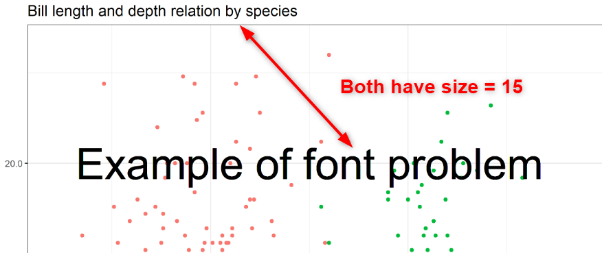
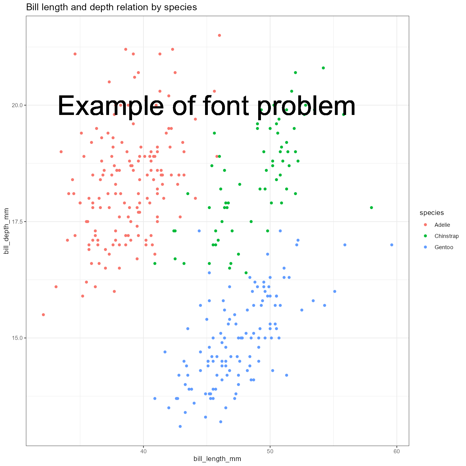
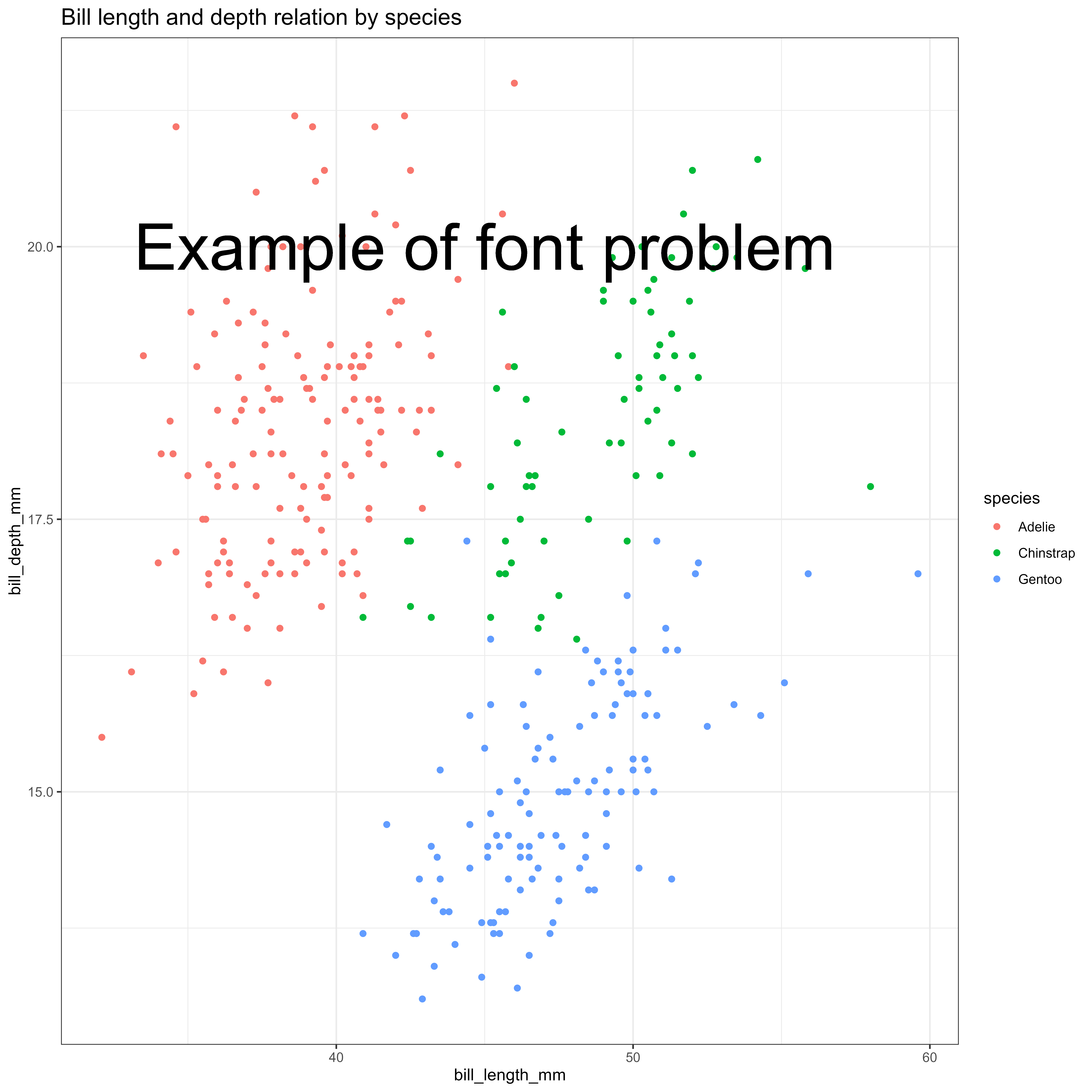
With this example, it become easier to understand a problem that occurs regularly when replicating a plot or changing the dimension or resolution, and can be confusing at first :
plt <- penguins %>%
  ggplot(aes(bill_length_mm, bill_depth_mm, color = species)) +
  geom_point()+
  geom_text(x = 45, y = 20, label = "Example of font problem", size = 15, inherit.aes = FALSE) +
  labs(title = "Bill length and depth relation by species") +
  theme(plot.title = element_text(size = 15))

ggsave("font_test2_10x10_300.png", plot = plt, width = 10, height = 10, units = "in", dpi = 300)

ggsave("font_test2_5x5_300.png", plot = plt, width = 5, height = 5, units = "in", dpi = 300)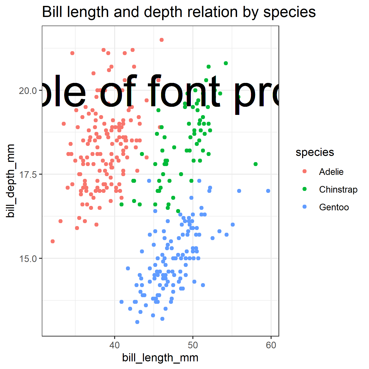
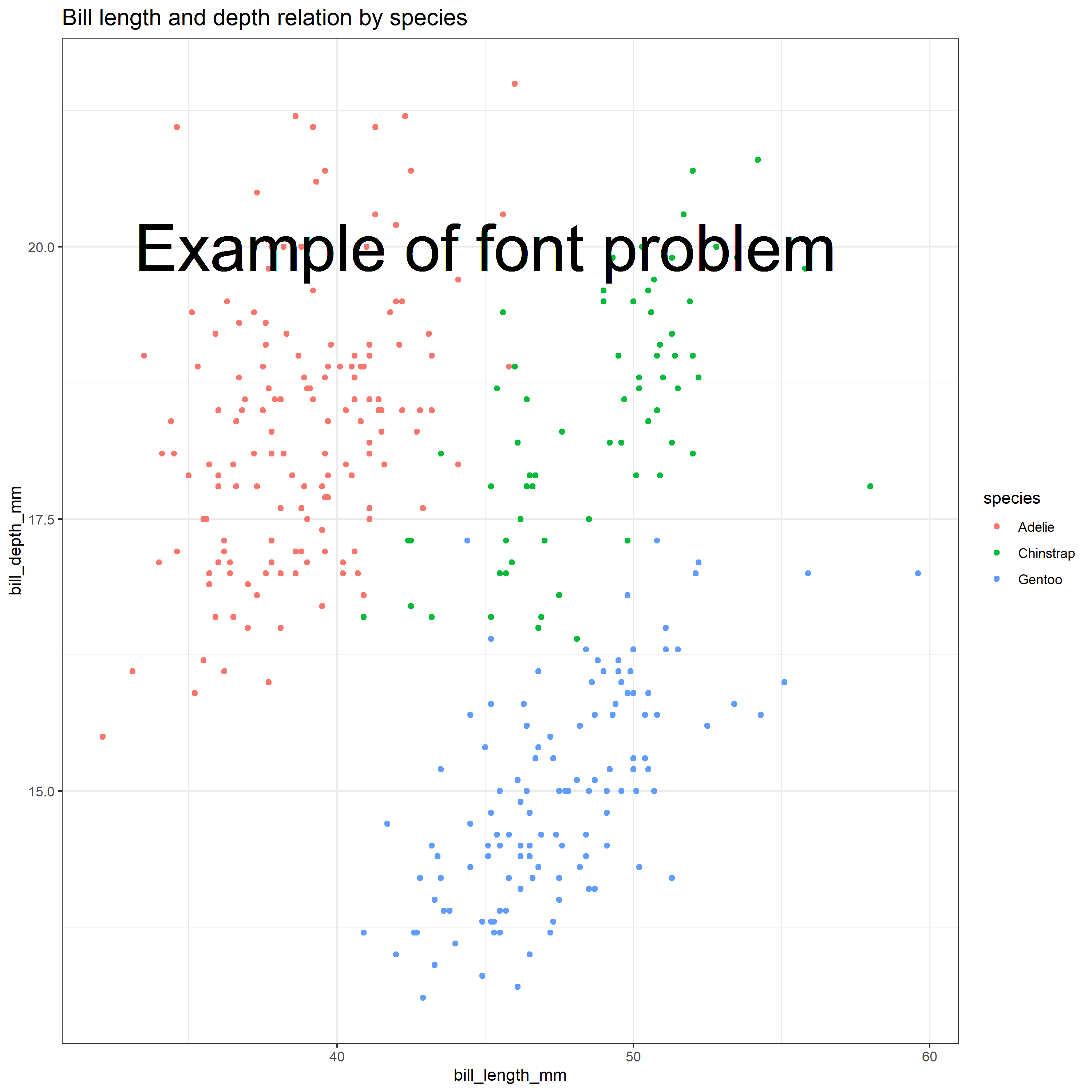
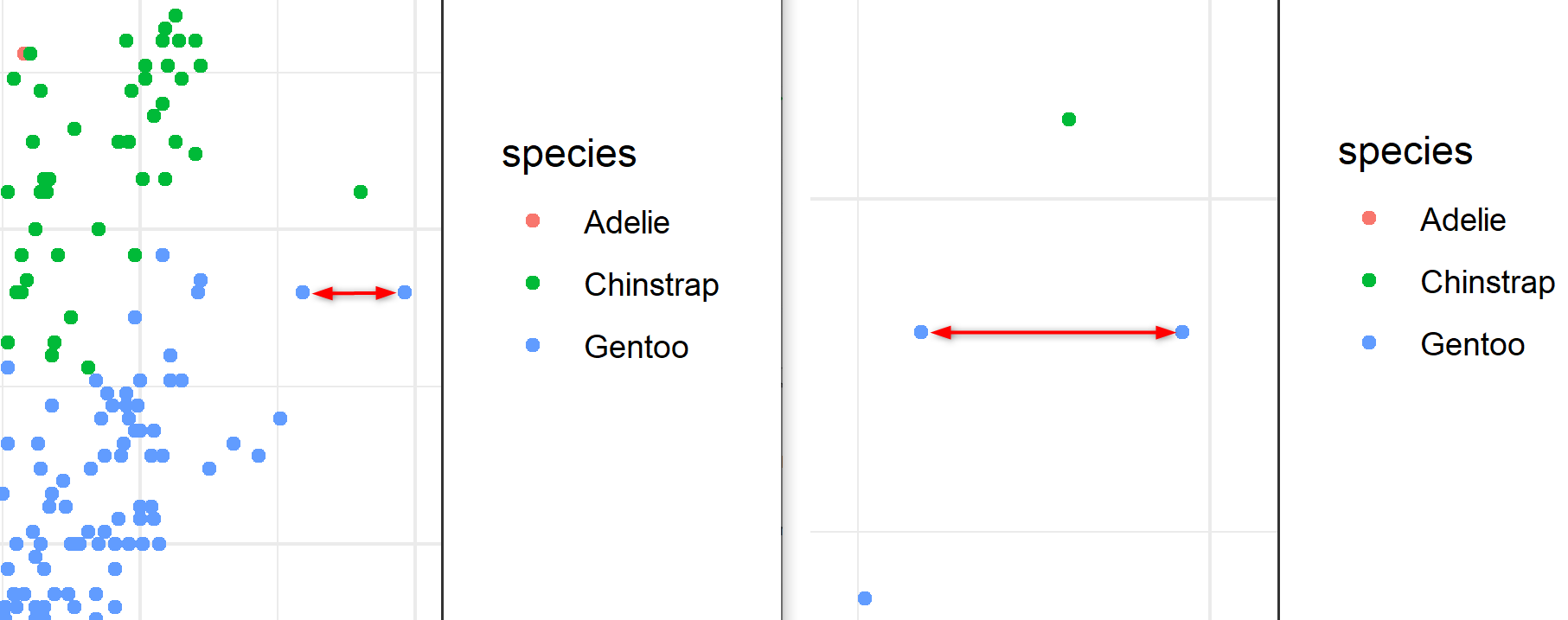
Here once again, the physical dimension of the font is the same (shown in the picture below with the actual physical dimension), but the plot size is different, so relatively, the text doesn’t fit anymore in the plot.
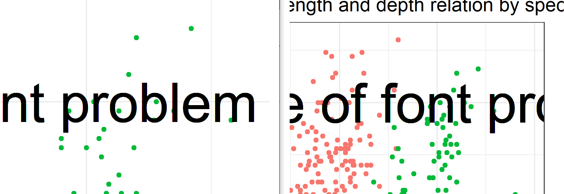
So there are 3 choices :
- Adjust the font size when you change your plot size or resolution, but if the plot is complex, that might involve a lot of modification.
- Set the size of the plot in inches and the resolution at beginning, and work on customization after.
- The ragg package have a scale parameter to handle the changes of dimension while keeping the proportions, see more detail at the end of the post.
The best option is to have this in mind, think about the proportion of your final visualization, and set the size of the plot before making complex customization with text and size. Knowing why this occurs it becomes easy to fix it when it happens, and chose the best option at that time.
Difference in font size
Maybe you noticed something else in the previous example, the text on the plot and the title both have a size of 15, but they look completely different. So why is that ?
In the theme, the size is defined in pts. So here 15, means 15 pts. In geom_text, the size is defined in mm, so it’s 15 mm.
What is the relation between pts and mm or in ? If we want exactly the same size for the title and the text in the plot, how can we define it ? It needs some conversion :
- 1 pt = 1/72 in
- 1 pt = 0.35 mm
So if we want the text to be the same size as the title, the size in mm will be 15 pt * 0.35 pt/mm = 5.25 mm
In ggplot, there is a constant defined to make the conversion, .pt = 2.845276. (1/.pt = 0.35). You can type in .pt in the console and it will display its value :
ggplot2::.pt## [1] 2.845276So to make the conversion :
- from pt to mm : mm = pt / .pt -> 15 / 2.845276 = 5.27
- from mm to pt : pt = mm * .pt -> 5.27 * 2.845276 = 15
Let’s change the size of the geom_text to be the same of the title by using size = 15/.pt :
plt <- penguins %>%
  ggplot(aes(bill_length_mm, bill_depth_mm, color = species)) +
  geom_point()+
  geom_text(x = 45, y = 20, label = "Example of font problem", size = 15/.pt, inherit.aes = FALSE) +
  labs(title = "Bill length and depth relation by species") +
  theme(plot.title = element_text(size = 15))

ggsave("font_title_10x10_300.png", plot = plt, width = 10, height = 10, units = "in", dpi = 300)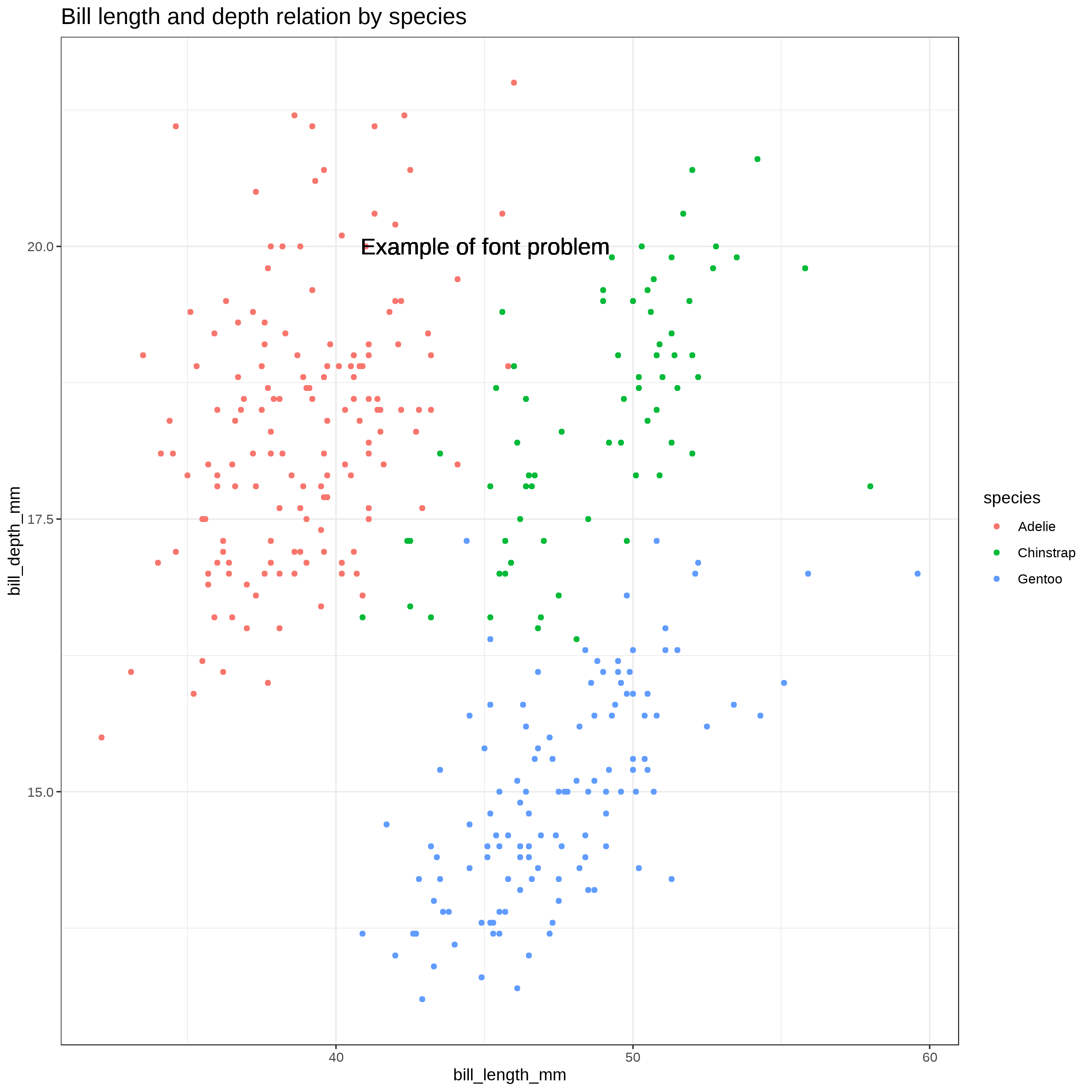
That’s it !
Example with showtext
Let’s do exactly the same plot, but using a different font with showtext.
library(showtext)

font_add_google("Roboto", "roboto")

showtext_auto(enable = TRUE)

plt <- penguins %>%
  ggplot(aes(bill_length_mm, bill_depth_mm, color = species)) +
  geom_point()+
  geom_text(x = 45, y = 20, label = "Example of font problem", size = 15/.pt, inherit.aes = FALSE) +
  labs(title = "Bill length and depth relation by species") +
  theme(plot.title = element_text(size = 15))

ggsave("showtext1_10x10_300.png", plot = plt, width = 10, height = 10, units = "in", dpi = 300)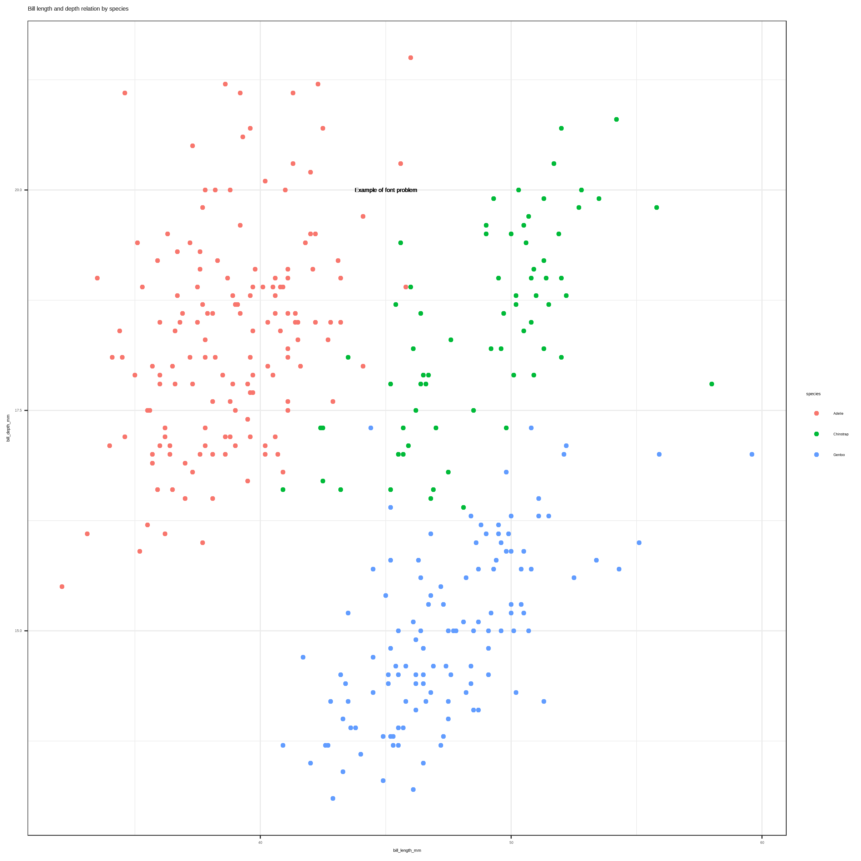
So what now ? I changed the font, and suddenly the text size is shrinking, I thought I understood, but am I still missing something ?
No, it’s same problem here. When calling showtext_auto(), the default text dpi is 96 ! We set our font size for the dpi we used in ggsave which was 300, but now the DPI used for the font is 96. So lets do the math, and first recall what we saw before, when saving a plot, we save a raster image which is a matrix of points :
The font that was 5.27mm at 300 dpi, which is 0.2074803 in * 300dpi = 62 dots The plot was 10 inches height, at 300 dpi = 3000 dots, so the text was 62 dots height on 3000 dots.
Now at 96 dpi, it’s 0.2075*96 = 20 dots, but the plot size is still 10 inches at 300 dpi. So relatively the text is now 20 dots height on 3000 dots height plot, which make it appear about 3 times smaller.
So I would recommend to set up all the options and fonts, before doing too much of the customization. But if you already did the customization when you decide to load a new font; the way to solve the problem is to tell showtext to use a DPI = 300 :
library(showtext)

font_add_google("Roboto", "roboto")

showtext_opts(dpi = 300)
showtext_auto(enable = TRUE)

plt <- penguins %>%
  ggplot(aes(bill_length_mm, bill_depth_mm, color = species)) +
  geom_point()+
  geom_text(x = 45, y = 20, label = "Example of font problem", size = 15/.pt, inherit.aes = FALSE) +
  labs(title = "Bill length and depth relation by species") +
  theme(plot.title = element_text(size = 15))

ggsave("showtext2_10x10_300.png", plot = plt, width = 10, height = 10, units = "in", dpi = 300)
Now it’s back to normal.
It’s something to consider when this happens, check the dimension and resolution, and see if there’s not a default value coming from a package.
Using the ragg package and scaling option
Now if you finished your plot, and you need to save to a different file dimension, you usually have to change the size of the font if you don’t want to face the previous problem, and some elements won’t keep the same dimensions or proportions, the point will look bigger or smaller, the distances between them won’t be the same.
The ragg package can help with that, it provide a parameter to scale the plot, for example, if we want to downsize our plot from 10x10 to 5x5 and want to keep the same proportion for the text, we can set the scaling option to 0.5.
plt <- penguins %>%
  ggplot(aes(bill_length_mm, bill_depth_mm, color = species)) +
  geom_point()+
  geom_text(x = 45, y = 20, label = "Example of font problem", size = 15/.pt, inherit.aes = FALSE) +
  labs(title = "Bill length and depth relation by species") +
  theme(plot.title = element_text(size = 15))

ragg::agg_png("ragg_10x10.png", width = 10, height = 10, units = "in", res = 300)
plt
dev.off()
ragg::agg_png("ragg_20x20.png", width = 20, height = 20, units = "in", res = 300, scaling = 2)
plt
dev.off()
ragg::agg_png("ragg_5x5.png", width = 5, height = 5, units = "in", res = 300, scaling = 0.5)
plt
dev.off()
These 3 files will have different dimension, but all the proportion will be conserved (click on them to see the real size).
Half size 5x5

Normal size 10x10
Double size 20x20
For a different explanation and more detail on how ragg solve the problem, you can look at this post Taking Control of Plot Scaling
Note that if you use agg_png as a type of device in ggsave, the scale argument doesn’t work anymore, it produces always the same image size, as if it divide the new size by the scaling (when I write this post, with version 0.4.1). So I recommand using it as a device like in the previous example.
Christophe Nicault
Information System Strategy
Digital Transformation
Data Science
I work on information system strategy, IT projects, and data science.